How Our Reverse Discounted Cash Flow Model Works
We make discounted cash flow (“DCF”) models easy and democratize the benefits of Expectations Investing.
See live Reverse DCF case studies in our private online community (use this form to sign up for free). In this case study, we apply our reverse DCF model to Nvidia (NVDA) at $120/share.
Bad DCF models are misleading. We won’t argue that, but DCF analysis remains extremely helpful when used to reverse engineer what companies have to do to justify their stock prices, aka expectations investing.
The right way to use DCF models is not try to predict the future, but to quantify the future that the stock price is predicting, aka expectations investing. You can get numerous real-world examples of how we use our reverse DCF and apply expectations investing to buy or sell decisions in all of our Danger Zone and Long Idea research.
Our DCF model differs from other DCF models in two ways:
- Unbiased – our DCF models tell us what the market is predicting.
- Better data – our DCF models use superior fundamental data, not analyst earnings or other flawed metrics.
First Principles: What Is A Reverse DCF Model?
Our DCF starts with the principle that stocks can be valued in the same way as bonds. As shown in Figure 1, the drivers of future cash flow between the two types of securities are analogous. The only difference is that the future cash flows for bonds are contractually determined while the future cash flows for stocks are undetermined. However, as long as one accepts the premise that the value of an asset equals the present value of future cash flows, then it follows that reverse DCF models can quantify the future cash flows required to justify stock prices.
Figure 1: The Basic Valuation Recipe: Same For Stocks And Bonds
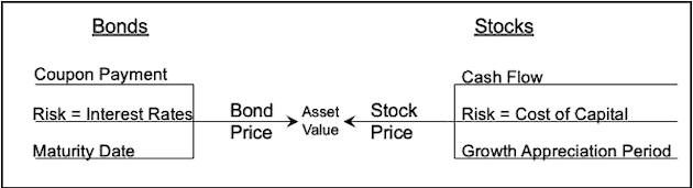
Sources: New Constructs, LLC and company filings.
In Figure 2, we categorize the drivers of a stock’s implied future cash flows into more intuitive terms.
Figure 2: Simpler Terms for Measuring Cash Flows
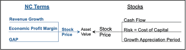
Sources: New Constructs, LLC and company filings.
We think it is easier to think about the future cash flows implied by stocks prices in these terms because they capture the core drivers of business success:
- Revenue Growth: how fast will the business grow?
- ROIC – WACC: how profitable with the business be?
- Growth Appreciation Period (GAP): for how long will the business grow profits?
In Figure 3, we match the more intuitive drivers for equity cash flows with the drivers of bonds. With this understanding, we can focus on using our reverse DCF to get the answers to these questions from Mr. Market.
Figure 3: The New Constructs Valuation Recipe: Same For Stocks And Bonds

Sources: New Constructs, LLC and company filings.
How the Reverse DCF Model Math Works
We start by providing a long forecast horizon for Revenue Growth and ROIC – WACC, not just five or 10 years (more details below). Then, we solve for the Growth Appreciation Period (GAP) needed for the DCF model to produce a stock price equal to the current stock price.
In other words, we provide forecasts for two of the three variables in the equation and solve for the 3rd variable. Users of our model can choose to solve for any of the three variables by entering forecasts for the other three. See the Appendix for details on the specific forecast inputs we use in our DCF models to forecast revenue, ROIC and WACC.
Our Reverse DCF Model Is Also “Dynamic”
Our DCF models do not rely on static forecast horizons such as five or ten years as do traditional DCF models. Our models are dynamic, which means we calculate values for the stock based on multiple forecast horizons. The key to this approach is a terminal value in each forecast horizon that assumes zero growth (e.g. NOPAT/WACC not WACC-g) after the forecast horizon. Rather than trying to capture all the future growth in cash flows in a static time frame (e.g. five years), our models calculate the value attributable to shareholders over multiple forecast horizons. For more details, see the reverse DCF case studies mentioned above.
Examples of Insights from Our Reverse DCF Models
Next, we share excerpts from our reports to show exactly how our models give investors important fundamental insight into the future cash flow expectations embedded in stock prices and how much risk they take owning stocks at certain prices.
- From our April 5, 2021 report Saving Investors from Meme Stocks: GameStop (GME):
“Crazy” Valuation at $347/share Explained: Implies More Revenue Than Macy’s
We use our reverse discounted cash flow (DCF) to show just how crazy the expectations implied by the peak valuation of GameStop. To justify $347/share, it shows that GameStop must:
- improve its profit margin to 5.5% (10-yr avg from 2010-19 is 3.9% & all-time high was 4.8% in 2008) and
- grow revenue by 17% compounded annually through 2030 (above projected video game industry CAGR of 13% through 2027)
In this scenario, GameStop earns nearly $21 billion in revenue in 2030 or more than the trailing-twelve-months (TTM) revenue of Macy’s (M), AutoZone (AZO), and Chewy Inc. (CHWY). For reference, GameStop’s revenue fell by 3% compounded annually from 2009 to 2019.
Figure 4: GameStop’s Historical Revenue vs. DCF Implied Revenue: Scenario 1
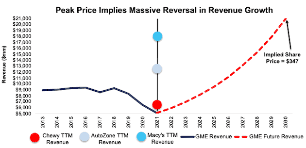
Sources: New Constructs, LLC and company filings
This analysis provides clear, objective perspective on just how ridiculous GME’s valuation was during the meme stock frenzy.
2. From our March 10, 2021 report The Real Winner of the Fintech Micro-Bubble:
Market Expectations Imply Square Wins the “Fintech Revolution” & JPMorgan Chase Will Lose
Below, we use our reverse discounted cash flow (DCF) model to highlight the disconnect in the future revenue and profit growth expectations baked into JPMorgan Chase’s and Square’s current stock prices.
To justify JPMorgan Chase’s current price of $152/share, we show that the market assumes:
- NOPAT margin falls to 26% (equal to its five-year average versus 31% TTM) and
- revenue falls 1% compounded annually for the next decade, which assumes revenue falls 3% in 2021, grows 3% in 2022 (equal to consensus estimates) and falls 1.5% a year each year thereafter.
In this scenario, JPMorgan Chase’s revenue ten years from now is $114.1 billion, or 12% below its 2020 revenue and nearly equal to its 2017 revenue. See the math behind this reverse DCF scenario.
On the other hand, to justify its current price of $225/share, Square must:
- immediately achieve a NOPAT margin of 5% (above its all-time high margin of 3.5%, compared to -1% TTM) and
- grow revenue by 37% compounded annually over the next ten years. For reference, average consensus estimates expect Square’s revenue to grow 23% compounded annually from 2021 to 2025.
Figure 5 compares the historical and implied future revenues implied by the current stock prices of JPMorgan Chase and Square.
Figure 5: Share Prices Imply Square’s Revenue Overtakes JP Morgan Chase’s
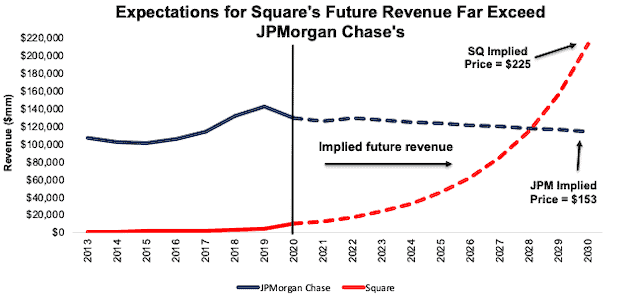
Sources: New Constructs, LLC and company filings.
In this scenario, Square’s revenue ten years from now is $213 billion, or 65% greater than JPMorgan Chase’s 2020 revenue and nearly 10-times greater than PayPal’s (PYPL) 2020 revenue. See the math behind this reverse DCF scenario.
This scenario implies that Square’s GPV in 2030 will equal $7.4 trillion, or 59% of all U.S. consumer spending in 2020[1].
Which stock do you think is attractively priced?
3. From our April 9, 2021 report Despite Record 1Q Results, Coinbase’s Valuation Remains Ridiculous:
Coinbase Is Priced to Be the Largest Exchange (by Revenue) in the World
When we use our reverse discounted cash flow (DCF) model to analyze the future cash flow expectations baked into Coinbase’s expected valuation, we find that shares are priced for beyond perfect execution.
In order to justify its expected $100 billion valuation, Coinbase must:
- maintain a 25% NOPAT margin (above Nasdaq’s 19% but below Intercontinental Exchanges’ 31% in 2020) and
- grow revenue by 50% compounded annually (well above Nasdaq’s highest seven-year revenue CAGR [2004-2011] of 30%) for the next seven years. See the math behind this reverse DCF scenario.
In this scenario, Coinbase would earn $21.3 billion in revenue by 2027, which would be 1.5x Intercontinental Exchange and Nasdaq’s combined 2020 revenue and nearly double Charles Schwab’s 2020 revenue.
Figure 6 compares the firm’s implied future revenue in this scenario to its historical revenue and the 2020 revenues of Intercontinental Exchange and Nasdaq combined as well as Schwab’s (SCHW) revenue in 2020.
Figure 6: Expected Valuation Implies Greater Revenue Than ICE & NDAQ Combined
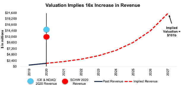
Sources: New Constructs, LLC and company filings
If Coinbase maintained its fees at 0.46% of trading volume (as outlined above), this scenario implies that trading volume on Coinbase’s platform would be $4.6 trillion by 2027, which would equal 97% of the total cryptocurrency trading volume in 2020.
The insights from our reverse DCF position investors to understand just how much risk they are taking when they buy stocks at certain levels. We are not saying that fundamentals should be 100% of your investing process. We only aim to add insight into the fundamental risk of owning stocks at different prices.
Appendix: The Inputs for Our “Dynamic” DCF Model
Below are the forecasting inputs for our DCF models along with explanations on how we derive our Default estimates for each input. Note that all of our models enable clients to change these inputs and create (and compare) as many future cash flow scenarios as they wish. See our tutorial on our Forecast page for more details on how to create and modify forecasts.
Forecast Driver #1: Revenue Growth
Revenue growth is the easiest of all the estimates. We like to base our Default forecasts on consensus revenue estimates for as many years as we can get them. Then, we tend to converge back to historical averages. From EY51-100, most of the time we assume a growth rate of 3% for all companies. We converge most companies to 3% over the long term because that is roughly the long-term geometric GDP growth rate since 1929.
These assumptions are only a baseline and can be adjusted as needed. Forecasted revenue growth should not be 6% if a company has never generated 6% growth, and our analysts make this adjustment in our Default forecasts.
Forecast Driver #2: Net Operating Profit Before Tax (NOPBT) Margin
Margin forecasts tend to be based on historical averages where they make sense. We prefer not to forecast significant deviations from what the company has done in the past. Also, the Default NOPBT margin forecasts tend not to change across the entire forecast period. This consistency simplifies measurement of the impact of differing margin level assumptions.
We cannot use consensus values for our margin forecasts because our margin calculations take into account a great deal more data than is used in most analysts’ models.
Forecast Driver #3: Cash Operating Tax Rate
Tax rate forecasts tend to be based on historical averages also. Like the margin forecast, tax rate forecasts tend not to change across the entire forecast period in our Default scenarios. By applying the cash operating tax rate to NOPBT, we get Net Operating Profit After Tax (NOPAT).
Forecast Driver #4: Changes in Invested Capital
To measure free cash flow, we must forecast how Invested Capital changes. We break out the Invested Capital forecasts into changes for net working capital and fixed assets. By forecasting the change in cash operating profits and the change in invested capital, we get both free cash flow and Return On Invested Capital (ROIC).
Forecast Driver #5: Weighted Average Cost of Capital (WACC)
The inputs above create a future stream of cash flows that we must discounted to their present to account for the opportunity cost of capital. We use the weighted-average cost of capital (WACC) to discount cash flows in each company model. Our WACC is based on standard formulas for calculating the cost of debt (risk-free rate plus a spread based on credit rating) and equity (CAPM). More details on WACC are here.
[1] In 4Q20, Square generated $929 million in transaction-based fees from $30.0 billion of GPV. We derive Square’s implied 2030 GPV of $7.4 trillion by dividing the firm’s implied 2030 revenue by its 4Q20 transaction-based fee rate of 2.9%. U.S. consumer spending in 2020 is estimated at $12.5 trillion.
Want To Learn More?
Sign up to receive free alerts about all our new research reports including Long Ideas and Danger Zone picks.
See our webinar on importance of ROIC and how to calculate it.
Get our report on "ROIC: The Paradigm For Linking Corporate Performance to Valuation."